SUBA5 Toolbox Help ¶

The SUBA5 toolbox is a new feature and more detailed description of each tool is currently in preparation for submission. However, this section will provide the user with the information and instruction necessary for use.

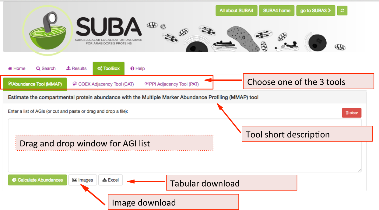
There are 3 tools available in the SUBA5 toolbox. The initial toolbox view shows the front of the MMAP protein abundance tool (tab is highlighted in green). Below the tab index, the heading contains a short description of the main feature of the tool that is currently chosen. To choose another tool e.g. the Coexpression Adjancency tool (CAT) , click on the CAT tab. All three tools have the AGI drag and drop window in common where AGIs can be dragged or pasted into. Besides tool-specific search functions, all tools have an image and tabular download function, which are situated underneath the AGI drag and drop window.

---

The Multiple Marker Abundance Profiling (MMAP) tool ¶

The MMAP tool has been developed to provide a method to estimate compartmental protein abundance without additional experimental data. The relative protein abundance for each protein was estimated from global aggregated and normalized mass spectrometry data in MASCP Gator https://omictools.com/mascp-gator-tool. A large number of marker proteins with high confidence was assembled for each compartment.

When submitting a list of AGIs through the drag-and-drop window, the marker proteins are identified from the list and the relative abundance is calculated for each compartment. The tool output shows the number of Arabidopsis proteins and the standard abundance distribution derived from all observed TAIR10 AGIs on the left and for the submitted user AGI list on the right, respectively. The tool also allows users to submit their own reference to calculate the abundance from.

Step by step instructions calculating an abundance distribution against the Arabidopsis standard ¶

This will calculate the abundance distribution/ enrichment in an AGI list submitted by the user when the starting material is unknown or a list of AGIs is not available for the starting material. By default the user-submitted list is compared to all available TAIR10 AGIs and their mass spectrometry data.

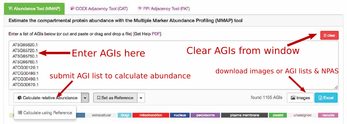
For using this option, paste a list of AGIs into the window. Once you press the calculate abundances button: 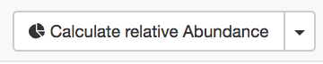you will receive the output. There are 4 bar graphs: two on the left (TAIR10 standard) and two on the right (user data).

Data interaction panel ¶

Subcellular category count and relative distribution data output panel

Standard (left 2 bars): The left bar graph shows the number of AGIs assigned to each compartment for all TAIR10 AGIs as per high confidence marker list. AGIs not assigned to compartments are in the category unassigned. The second left bar graph shows the abundance distribution across the standard data sets of all integrated mass spectrometry data for the TAIR10 proteome.

The user submitted data (right 2 bars): The third bar graph from the left shows the number of AGIs in each compartment for the user-submitted list of AGIs according to hits in the HCM list (The user AGI list is compared to the HCM list and the hits are being identified and summed per compartment). The right bar graph shows the calculated abundance distribution in the user-submitted sample and normalizes is to the total of 1 (relative abundance distribution of organellar protein in the user sample). This will show any enrichment of organellar protein.

In the mouse over, both abundance distribution bar graphs show a minimum and maximum range of NPAS for each compartment as well as the average abundance as a fraction of 1 and in percentage, respectively.

Step by step instructions setting a custom reference and calculating an abundance distribution against the custom reference ¶

Short cut instructions ¶

1. Enter the list of AGIs you want to use as your reference into the window
2. Press “Calculate relative Abundance”
3. Press “Set as Reference”
4. Clear reference AGIs from the window
5. Enter your list of AGIs for assessing against the reference into the window
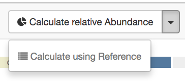
6. Press the arrow down next to “Calculate relative Abundances” and choose “Calculate using Reference”

---

Detailed instructions ¶

For estimating the enrichment of a sample against your own reference data set, you have to set the reference first. Enter the list of AGIs you want to use as your reference into the window and press the “Calculate relative Abundance” button.

The bar graphs on the right side will display the compartmental AGI count and abundances for your reference set. Now press the “Set as Reference” button to save this data. Set the abundance distribtution as your reference.

---

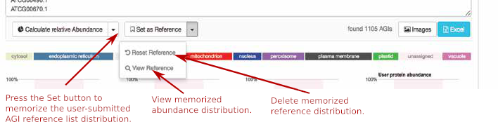
To clear or view the reference activate the arrow next to the “Set as Reference” button to get to the “Reset Reference” and “View Reference” option. The “View Reference” will show you the raw NPAS sums for each compartment in your reference AGI list.

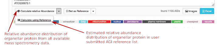
You can now clear the AGIs from the window and add your AGI list that you want to investigate. On the right side of the “Calculate relative Abundance” button is an arrow that will drop down into the “Calculate using Reference” button. Now you can choose to calculate your entered AGI list comparing it to your reference that you set earlier or if you click on the “Calculate relative Abundance” button you can calculate it against the TAIR10 standard. The bar graphs on the right will display the results of either.

---

The Coexpression Adjacency Tool (CAT) ¶

The coexpression adjacency tool provides spatial analysis statistics for coexpression partners using SUBAcon location calls. The user can drag a list of AGIs in the window on the top and look for coexpressed AGIs either within the list (‘restrict to my list’) or globally. SUBA5 contains the top 300 coexpressed partners and excludes self-coexpressed AGIs (rank = 1). Pressing the ‘Find coexpressed proteins’ or the ‘restrict to my list’ button submits the query and returns the statistics.

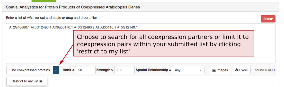
To limit the list of coexpressed partners, the coexpression rank (mutual rank 2-300) and strength (average coexpression coefficient 0-1) can be restricted. The list of coexpressed AGIs can also be filtered by the spatial relationship of the expressed proteins. The categories include matching, adjacent, distant location pairing as well as secretory for locations exclusively within ER, Golgi, vacuole, plasma membrane and extracellular. Mixed location calls with unclear biological implications are combined into the category unclear.

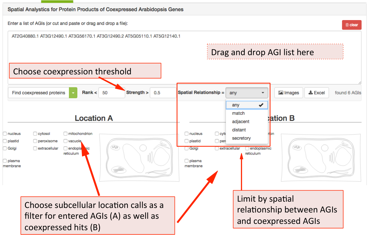
When searching for specific location pairings, the user-submitted list of AGIs can also be specifically limited to location calls for the proteins submitted (location A) and the location calls for the coexpressed proteins (location B).

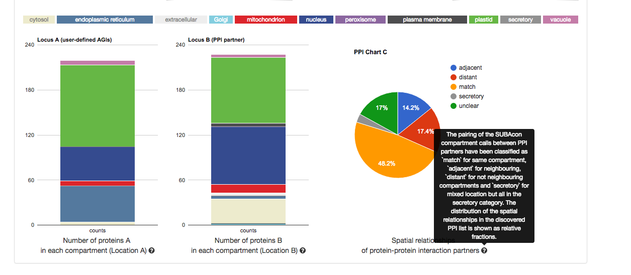
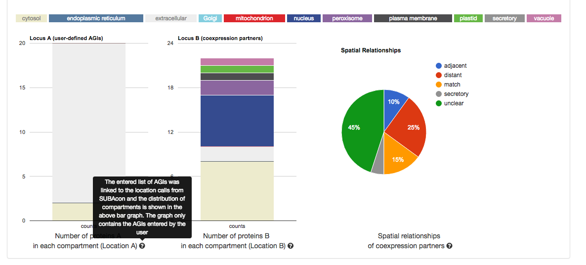
Once submitted, the statistics for your user list will appear in format of 3 graphs. From left to right, it shows the distribution of the location calls for the user-submitted AGIs (Location A) and the distribution of the location calls for the retrieved coexpressed AGIs (Location B). If the ‘restrict to my list’ option was chosen, these distributions may look very similar. The pie chart on the right shows the distribution of the spatial relationships of the coexpression couples. This relative measure shows the % of matching, adjacent and distant compartment PPIs. The information for each graph can be obtained by gliding over the question mark behind the x-Axis title below the graph.

---

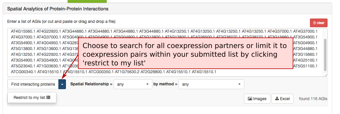
The PPI Adjacency Tool (PAT) ¶

The Protein-Protein Interaction (PPI) adjacency tool provides spatial analysis statistics for PPI partners using SUBAcon location calls. The user can drag a list of AGIs in the window on the top and look for PPI partners either within the list. (‘restrict to my list’) or globally. SUBA5 contains a set of experimentally verified PPI proteins that is searched through this tool. Pressing the ‘Find interacting proteins’ or the ‘restrict to my list’ button submits the query and returns the statistics.

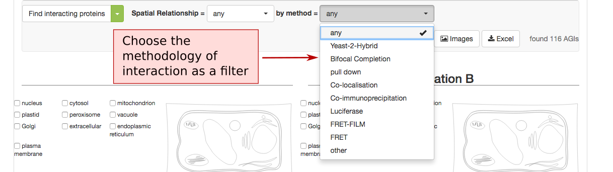
The PPI retrieval can be limited by the locations in two different ways. Firstly the user can choose to only view PPI proteins which have PPI partners in the same (match), neighbouring (adjacent) or non-neighbouring (distant) compartments. For PPI partners within the secretory but not matching (e.g. ER – Golgi), the category ‘secretory’ was introduced. This may help identify functionally related proteins within the PPI cohort.

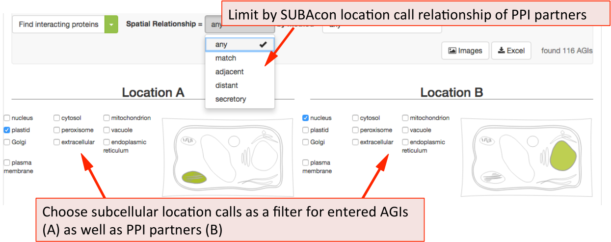
The list of proteins can also be refined using the type of methodology that was used to identify the PPI. This includes Yeast-2-hybrid, immune co-precipitation, bifocal completion and other methodologies that can be chosen from the drop down menu.

Once submitted, the statistics for your user list will appear in format of 3 graphs. From left to right, it shows the distribution of the location calls for the user-submitted AGIs (Location A) and the distribution of the location calls for the retrieved PPI AGIs (Location B). If the ‘restrict to my list’ option was chosen, these distributions may look very similar. The pie chart on the right shows the distribution of the spatial relationships of the PPI couples. This relative measure shows the % of matching, adjacent and distant compartment PPIs. The information for each graph can be obtained by gliding over the question mark behind the x-Axis title below the graph.